

1.10. Plotting Functions and Visualising Models#
It can often be useful to visualise mathematical functions. In order to plot
mathematical functions using line plots we need to obtain the corresponding
\(x\) and \(y\) values. One of the easiest ways to do this is to
generate a range of \(x\) values using the numpy function linspace.
First we need to import numpy.
import numpy as np
Then we use linspace to create an array of equally spaces values that lie
between the start and end values specified.
np.linspace(start, end, number of values)
The following creates an array containing 10 values between 2 and 4 (inclusive).
import numpy as np

print(np.linspace(2, 4, 10))
To create the corresponding \(y\) values we apply our function to \(x\), then we plot the results!
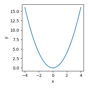
Example: Here we plot the function \(y = x^2\) to the values of \(x\) between -4 and 4.
import numpy as np
import matplotlib.pyplot as plt

x = np.linspace(-4, 4, 100)
y = x**2

plt.figure(figsize=(3, 3))
plt.plot(x, y)
plt.xlabel("x")
plt.ylabel("y")
plt.tight_layout()
plt.savefig("plot.png")
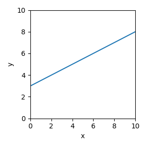
Example: Here we plot the function \(y = 0.5x + 3\) to the values of \(x\) between 0 and 10.
import numpy as np
import matplotlib.pyplot as plt

x = np.linspace(0, 10, 100)
y = 0.5 * x + 3

plt.figure(figsize=(3, 3))
plt.plot(x, y)
plt.xlabel("x")
plt.ylabel("y")
plt.xlim([0, 10])
plt.ylim([0, 10])
plt.tight_layout()
plt.savefig("plot.png")
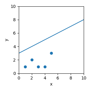
Scatter plots and line plots can be added to the same figure, we just use one command after the other.
import numpy as np
import matplotlib.pyplot as plt

x_points = np.array([1, 2, 3, 4, 5])
y_points = np.array([1, 2, 1, 1, 3])

x_line = np.linspace(0, 10, 100)
y_line = 0.5 * x_line + 3

plt.figure(figsize=(3, 3))
plt.scatter(x_points, y_points)
plt.plot(x_line, y_line)
plt.xlabel("x")
plt.ylabel("y")
plt.xlim([0, 10])
plt.ylim([0, 10])
plt.tight_layout()
plt.savefig("plot.png")
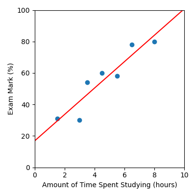
Now let’s put this all together to visualise the model we built on our study dataset. Here is a list of all the steps we’ve carried out.
Load the csv dataset into numpy arrays
Build a linear regression model using sklearn
Extract out the intercept and gradient from our linear regression model
Calculate the \(x\) and \(y\) values to plot the function associated with the linear regression model
Produce a figure that plots:
The data as a scatter plot
The linear regression model as a line
Here is the corresponding code:
from sklearn.linear_model import LinearRegression
import matplotlib.pyplot as plt
import pandas as pd
import numpy as np

# Load data
data = pd.read_csv("study.csv")
x = data["Time Spent Studying (hours)"].to_numpy()
y = data["Exam Mark (%)"].to_numpy()

# Build linear regression model
linear_reg = LinearRegression()
linear_reg.fit(x.reshape(-1, 1), y)

intercept = linear_reg.intercept_
gradient = linear_reg.coef_[0]

# Create x and y values to visualise the model function
x_model = np.linspace(0, 10, 50)
y_model = gradient * x_model + intercept

# Visualise the results
plt.figure(figsize=(4, 4))
plt.scatter(x, y)  # Data
plt.plot(x_model, y_model, color="red")  # Model
plt.xlabel("Amount of Time Spent Studying (hours)")
plt.ylabel("Exam Mark (%)")
plt.xlim([0, 10])
plt.ylim([0, 100])
plt.tight_layout()
plt.savefig("plot.png")
Code Challenge: Visualise a Linear Regresion Model
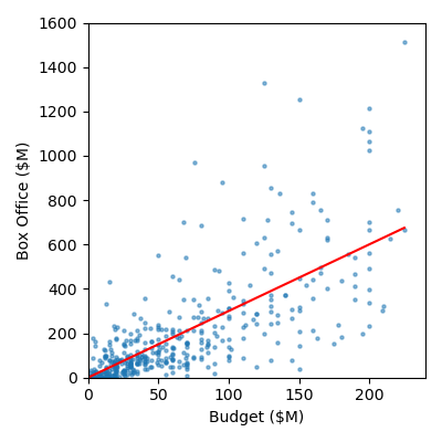
Now we’ll visualise the linear regression model we just built on our movie data. movie.csv
Instructions
You will need to combine the code you have written in the previous challenge Fitting a Linear Regression Model to:
Load the csv dataset into numpy arrays
Build a linear regression model using
sklearnExtract out the intercept and gradient from our linear regression model
Then you will need to
Calculate the x and y values to plot the function associated with the linear regression model
Use
np.linspace(0, 225, 50)to create the x values
Produce a figure that:
Plots the data as a scatter plot, marker size = 5 and alpha = 0.5
Plots the linear regression model as a line, in red
Has labels Budget ($M) and Box Office ($M)
Has x limits: 0 to 240
Has y limits: 0 to 1600
Your plot should look like this:
Solution
Solution is locked